NBA Player Insights: EDA & Performance Prediction

This project explores a rich dataset of NBA player statistics to perform an in-depth Exploratory Data Analysis (EDA), identify key performance drivers, and develop a machine learning model to predict career points per game. The analysis showcases a full data science workflow, from data wrangling and visualization to SQL querying and predictive modeling, using Python and its powerful ecosystem.

Project Objectives

To meticulously clean and preprocess raw NBA player statistics.
To conduct comprehensive EDA to reveal patterns in player performance, draft outcomes, physical attributes, and origins (college/country).
To demonstrate SQL proficiency for targeted data analysis within a Python environment using `pandasql`.
To build and evaluate regression models predicting a player's career points per game (PTS) based on pre-NBA characteristics.
To interpret model results, highlighting key predictive features and discussing limitations.

1. Data Wrangling & Preparation

The foundation of any robust analysis is clean data. The initial phase involved loading the `PlayerIndex_nba_stats.csv` dataset (sourced from official NBA statistics) and systematically addressing data quality:

Handling Missing Data: Imputed missing values appropriately for both categorical (e.g., 'Unknown' for `POSITION`, `COLLEGE`) and numerical attributes (e.g., 0 for `PTS`, `REB`, `AST` for EDA purposes where missing implies no recorded stat).
Data Type Conversion: Transformed fields like player `HEIGHT` (e.g., "6-10") into numerical inches and `WEIGHT` into numeric pounds, handling non-standard entries.
Feature Engineering: Created composite features like `PLAYER_NAME` and a boolean `IS_UNDRAFTED` flag from draft information.

# Example: Converting height to inches
def height_to_inches(height_str):
    if pd.isna(height_str) or not isinstance(height_str, str) or '-' not in height_str:
        return np.nan
    # ... (rest of function from your notebook) ...
    df['HEIGHT_INCHES'] = df['HEIGHT'].apply(height_to_inches)

# Example: Creating IS_UNDRAFTED flag

df['IS_UNDRAFTED'] = df['DRAFT_NUMBER'].isnull()

2. Exploratory Data Analysis (EDA) - Key Insights

Visualizations were key to understanding the data's nuances. Some highlight findings include:

Player Performance Landscape: Core stats (PTS, REB, AST) showed right-skewed distributions, with elite players significantly outperforming the average.

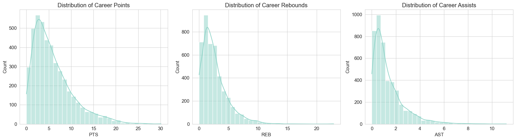
Career Points Distribution

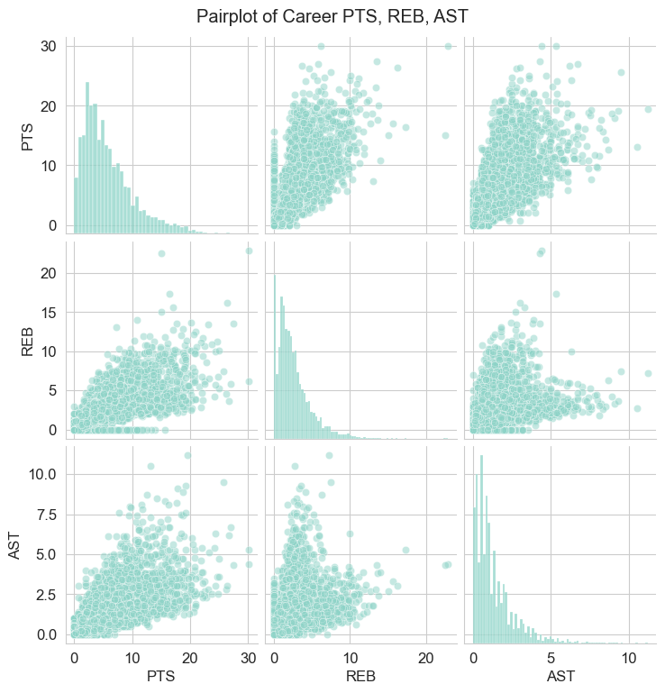
Correlations between PTS, REB, AST
Positional Variances: Guards excelled in assists, while Centers/Forwards dominated rebounds and height. Forward-Guards in this dataset showed high average points.

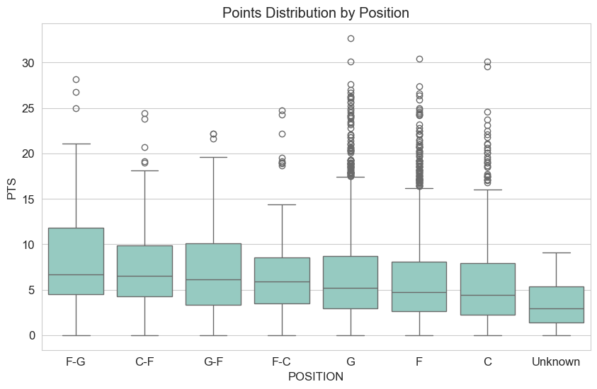
Points by Position

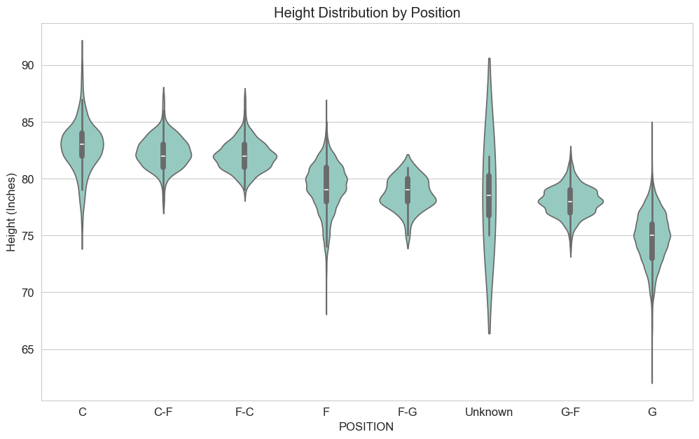
Height by Position
Draft Impact: Earlier draft picks (lower `DRAFT_NUMBER`) strongly correlated with higher career average points. First-round draftees averaged significantly more career PTS than later-round picks.

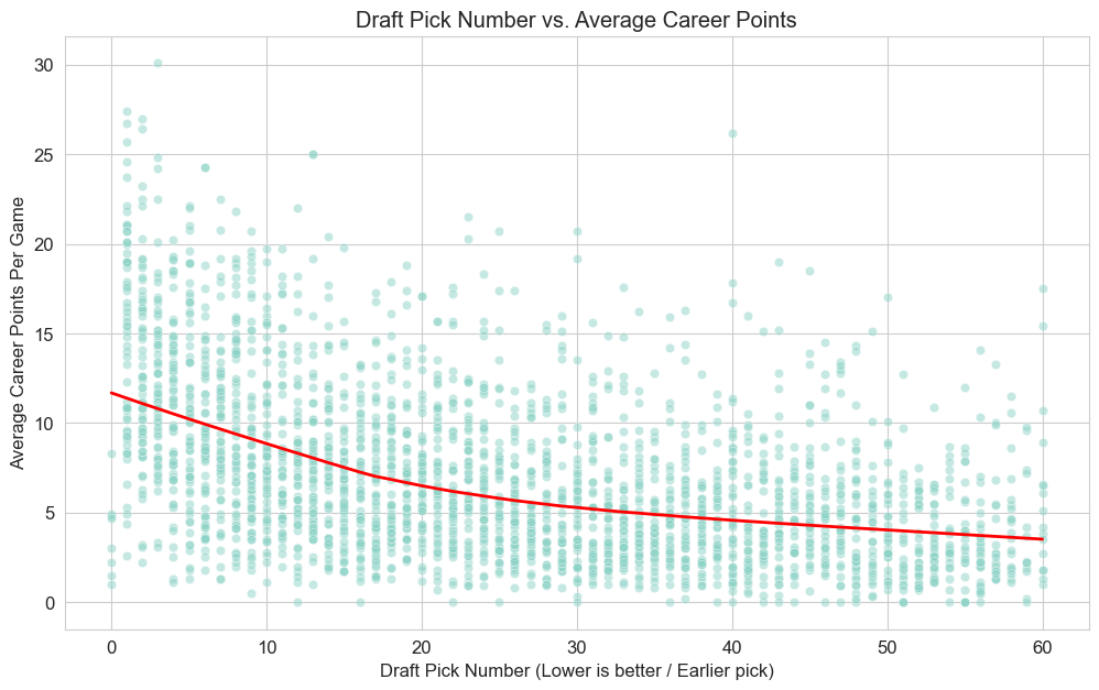
Draft Pick vs. Career Points (Lower pick number is better)

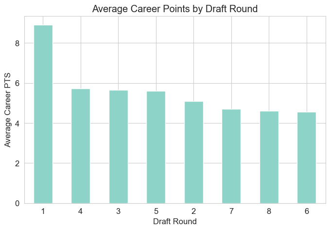
Average Career PTS by Draft Round
College & International Pipelines: Powerhouse NCAA programs (Kentucky, UCLA, Duke) are major talent sources. Internationally, Canada, France, and Serbia lead in representation, with players from Spain and Croatia showing strong scoring averages.

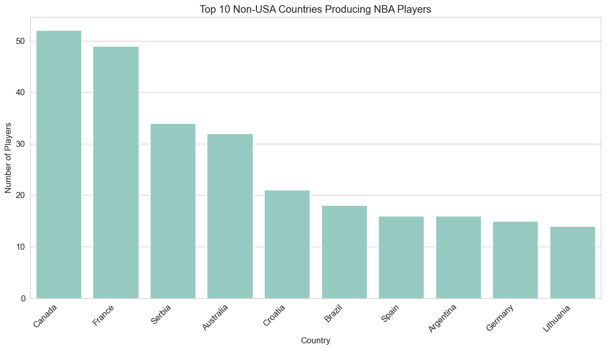
Top Non-USA Countries by Player Count

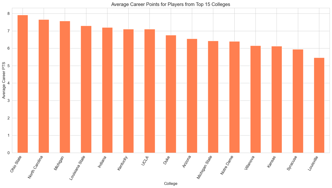
Average Career PTS: Top 15 Colleges

3. SQL for Targeted Analysis (via `pandasql`)

To demonstrate versatile data retrieval, SQL queries were executed on Pandas DataFrames using `pandasql`. This allowed for analyses such as:

Identifying Top 10 career scorers.
Calculating average PTS by player position.
Filtering for high-performing alumni from specific colleges (e.g., Duke players >15 career PPG).

-- Example: Duke Players with > 15 Career PPG
SELECT PLAYER_NAME, COLLEGE, PTS
FROM career_df
WHERE COLLEGE = 'Duke' AND PTS > 15
ORDER BY PTS DESC;

This approach combines Python's analytical power with SQL's declarative querying strength.

4. Predictive Modeling: Career Points Per Game (PTS)

A machine learning model was developed to predict a player's career average PTS using features like `DRAFT_NUMBER`, `DRAFT_ROUND`, `HEIGHT_INCHES`, `WEIGHT_LBS`, `POSITION`, and `COLLEGE`.

Preprocessing: Involved median imputation and StandardScaler for numerical features, and 'Unknown' imputation followed by OneHotEncoding for categorical features.
Models Evaluated: Linear Regression, Ridge Regression, Random Forest Regressor, and Gradient Boosting Regressor.
Best Model Performance: The **Random Forest Regressor** yielded the most promising results:
- R-squared (R²): ≈ 0.252 (explaining about 25.2% of the variance in career PTS)
- Root Mean Squared Error (RMSE): ≈ 3.99 points
Key Feature Importances (from Random Forest):
1. `DRAFT_NUMBER` (overwhelmingly most significant)
2. `HEIGHT_INCHES`
3. `WEIGHT_LBS`
4. `DRAFT_ROUND`
Specific positions and colleges also appeared, though their individual impact was more diffused.

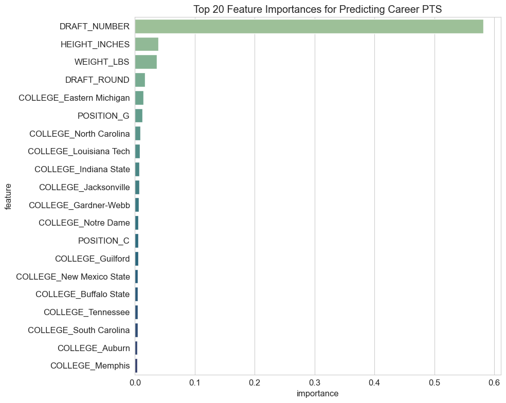
Top Feature Importances for Career PTS Prediction.
Model Limitations: The model serves as an exploratory tool. Its predictive power is constrained by the inherent randomness in player development, uncaptured intangible factors (work ethic, injuries), and the granularity of predicting career averages.

Dashboarding Potential with Power BI

The cleaned and analyzed dataset is ideal for developing interactive Power BI dashboards. Conceptual dashboards could include:

Player Profile Explorer: Deep dive into individual player stats and career trajectories.
Draft Class ROI Analysis: Evaluate draft success by position and pick number.
Geospatial Talent Mapping: Visualize player origins and performance hotspots.
"What-if" Predictive Scenarios: (Conceptual) Input player attributes to see model-based PTS predictions.

View Notebook & Code on GitHub » View HTML Notebook Preview »